Chapter Objectives
After reading this chapter, you'll be able to do the following:
Create a variety of curves and surfaces
Trim areas of NURBS surfaces
Use NURBS profiles to specify the beveled edges of 3D text
(Advanced)
Curves and curved surfaces provide a convenient mathematical means of describing a geometric model. Instead of using drawings, metal strips, or clay models, designers can use these mathematical expressions to represent the surfaces used on airplane wings, automobile bodies, machine parts, or other smooth curves and surfaces. Inventor uses a particular type of parametric polynomial, a NURBS (Non-Uniform Rational B-Spline), to represent curves and surfaces. This entire chapter can be considered advanced material.
To use NURBS curves and surfaces in an Inventor program, you need to develop an intuitive feel for a number of basic concepts. This section defines these key concepts and shows how they pertain to the various Inventor NURBS-related classes. For a more rigorous mathematical description of a NURBS, see “Suggestions for Further Reading” at the end of this chapter.
This chapter describes use of the following classes:
For simplicity, this discussion first explains the important NURBS concepts in terms of curves, which are lines in 3D space, such as a helix. Once you understand how to define a NURBS curve, defining a NURBS surface is a simple extension of your knowledge (see “NURBS Surfaces”).
A NURBS curve or surface is parametric—that is, the equations that describe it depend on variables (or parameters) that are not explicitly part of the geometry. A NURBS curve is described in terms of one parameter, u. The following three functions map this single parameter into x-y-z space:
x = f(u) y = g(u) z = h(u) |
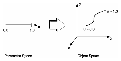
By sweeping through different values of u (that is, through parameter space), it is possible to evaluate the equations and determine the x, y, and z values for points on the curve in object space. Figure 8-1 represents this mapping of parameter space to object space.
Your job as programmer is to define the components that make up the parametric functions, referred to as f(), g(), and h() in the previous section. Instead of explicitly specifying the equations, you specify the following three things:
Control points—using SoCoordinate3 or SoCoordinate4 nodes
Knot sequence—using SoNurbsCurve or SoIndexedNurbsCurve nodes
Order—implicitly defined by number of control points and number of knots
A brief description of each is provided in this section, along with discussions of how they are related and how continuity is defined. A more elaborate description is provided in “Basis Function”.
Control points are points in object space that affect the shape of the curve in some way. The curve may pass near the control points, as shown at the left in Figure 8-2, or pass through some of them, as shown at the right in the figure. The control points can be a set of data points through which you want to fit a curve, or a grid of points used to describe a curved surface such as the hood of a car. In Inventor, control points are specified in an SoCoordinate3 or SoCoordinate4 node.
The knot sequence defines how the control points affect the curve. The knot sequence is simply a list of nondecreasing numbers. These numbers determine whether the curve passes through and interpolates between some of the control points (an interpolating curve) or passes near the control points (an approximating curve). In Inventor, the knot sequence is specified in an SoNurbsCurve or SoNurbsSurface (or SoIndexedNurbsCurve, SoIndexedNurbsSurface) node.
The order of a curve determines the form of the parametric equations. The order is equal to one plus the maximum exponent (degree) of the variables in the parametric equations. For example, the parametric equations of a cubic curve (degree = 3, order = 4) have the following form:
x(u) = Axu3 + Bxu2 + Cxu + Dx y(u) = Ayu3 + Byu2 + Cyu + Dy z(u) = Azu3 + Bzu2 + Czu + Dz |
Similarly, the parametric equations of a quadratic curve (degree = 2,
order = 3) have the following form:
x(u) = Axu2 + Bxu + Cx y(u) = Ayu2 + Byu + Cy z(u) = Azu2 + Bzu + Cz |
Alternatively, you may wish to think of the order as the number of coefficients in the parametric equation. The order of a curve affects how smooth the curve can be (see “Continuity of a Curve”).
In Inventor, the order of a curve is not explicily specified. Order is equal to
number_of_knots - number_of_control_points
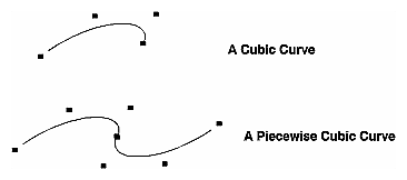
The order of the curve determines the minimum number of control points necessary to define the curve. You must have at least order control points to define a curve. (So for a curve of order 4, you must have at least four control points.) To make curves with more than order control points, you can join two or more curve segments into a piecewise curve (see Figure 8-3).
The order of the curve also affects how the curve behaves when a control
point is moved. In Inventor, a NURBS curve can have an order up to 8. However, higher orders introduce oscillation into the curve and can behave unpredictably when a control point moves. Cubic curves (order of 4) are the most commonly used curves, since they provide enough control for most geometric modeling applications without the drawbacks of higher-order curves.
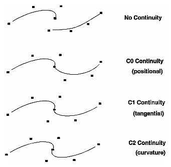
A breakpoint is where two curve segments meet within a piecewise curve. The continuity of a curve at a breakpoint describes how those curves meet at the breakpoint. Figure 8-4 shows four possible types of continuity:
The order of a curve determines the maximum continuity possible. Thus, you may need a higher order curve if you need more continuity. The maximum continuity is order - 2. For example, for cubic curves, the maximum continuity possible is C2 (curvature continuity).
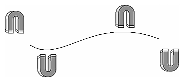
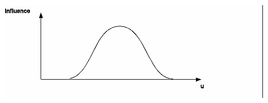
Each control point is like a magnet tugging on the curve (see Figure 8-5). The strength and extent of these magnets is described mathematically by a particular basis function. For a NURBS, this function is the B-spline basis function. (See “Suggestions for Further Reading” for references presenting a more thorough derivation of the B-spline basis function.)
The B-spline basis function (Figure 8-6) describes the curve in parameter (u) space. For each value of u:
contribution_of_each_control_point = location * its_basis _function
The resulting curve is equal to the sum of the contributions from each control point. Note that often a control point (a “magnet”) affects the entire curve, although its influence becomes weaker as you move away from it. The exact extent of the influence is determined by the knot sequence.
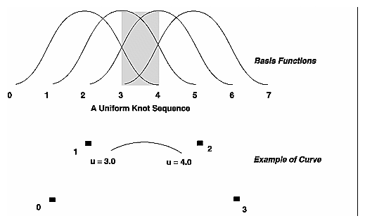
The distribution of basis functions in parameter space is controlled by the knot sequence (also referred to as the knot vector, or the knots). The knot sequence is a list of nondecreasing values. Each knot defines the beginning and end of a basis function. There must be exactly (order + number of control points) values in the knot sequence. The curve is defined only where order basis functions overlap (as shown in Figure 8-7). If the knot values are singular (no repeating values) and regularly spaced, the curve is a uniform B-spline (as shown in Figure 8-7).
Figure 8-7 shows a uniform knot sequence. Four control points are defined (in object space). The top of the figure illustrates the four basis functions for each of the control points. The basis functions overlap where u = 3.0 to
u = 4.0, as indicated by the shaded portion. This figure also illustrates another important NURBS relationship: at any point where the curve is defined, the sum of all basis functions is equal to 1.
Distinct knot values define segments. A basis function always spans order segments. In Figure 8-7, for example, the basis function beginning at 0 and ending at 4 spans four segments (knot 0 to knot 1; knot 1 to knot 2; knot 2 to knot 3; and knot 3 to knot 4).
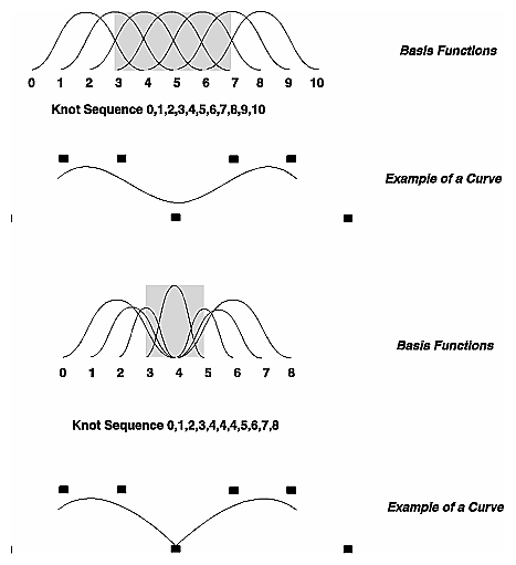
Duplicating values in the knot sequence increases that value's multiplicity and causes more than one basis function to start at that point. This also causes a corresponding decrease in the continuity of the curve. Figure 8-8 uses the same two sets of control points, with different knot sequences for the top and bottom curves. Notice how the bottom curve has C0 continuity, and the top curve has C2 continuity. This relationship between multiplicity and the continuity of the curve can be expressed mathematically as follows:
CORD - (M + 1) |
where ORD equals the order of the curve and M is the multiplicity.
The maximum multiplicity (maximum times you can repeat a knot) is order. Table 8-1 shows knot multiplicity and the resulting continuity.
Table 8-1. Continuity and Knot Multiplicity for Cubic Curves
Knot Multiplicity | Continuity | Continuity |
|---|---|---|
1 | positional | C2 |
2 | positional | C1 |
3 | positional | C0 |
4 | none | none |
Several common knot sequences are extremely useful for a wide variety of applications:
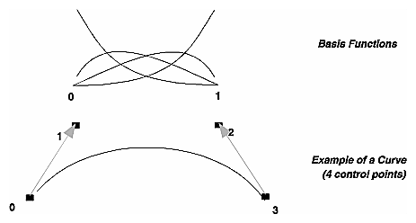
The behavior of the Bezier curve and the uniform cubic B-spline makes them ideal for geometric modeling and CAD applications. The curve passes through the first and last control points (see Figure 8-9). A line drawn through the first and second control points determines the tangent at the first endpoint. A line drawn through the last two control points determines the tangent at the second endpoint.
The previous pages have outlined important relationships among NURBS parameters. They can be summarized as follows:
Thus, for cubic curves, the order equals 4. You need at least four control points to define a cubic curve. The maximum continuity for cubics is C2 continuity. You need a minimum of eight knots in the knot sequence. The maximum knot multiplicity of cubics is 4.
Each control point has an associated weight that influences the shape of its basis function. As shown in Figure 8-10, this is analogous to having magnets of differing sizes tugging on the curve. For nonrational curves, all control points have a weight of 1.0. For rational curves, the control points have differing weights. If a control point has a weight greater than 1.0, its influence on the curve is greater than that of control points with weights
of 1.0.
The parametric equations for rational curves have both a numerator and a denominator, which results in a ratio. (The numerator is the original parametric equation. The denominator is another parametric equation that takes the weight into account.) We recommend that the weight be a value greater than 0. Use an SoCoordinate4 node to specify x, y, z, and w (weight) values.
Rational curves and surfaces are required to accurately represent conic sections, spheres, and cylinders. For more information, see “Suggestions for Further Reading”.
This section provides two examples of NURBS curves: a B-spline curve and a uniform B-spline curve that passes through the end control points.
Example 8-1 creates and displays a B-spline curve. Seven control points are defined. The knot vector contains ten knots. Since
number_of_knots = order + number_of_control_points |
this curve has an order of 3. It has a multiplicity of 2 (one knot is used twice). This curve has a continuity of C0.
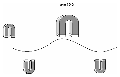
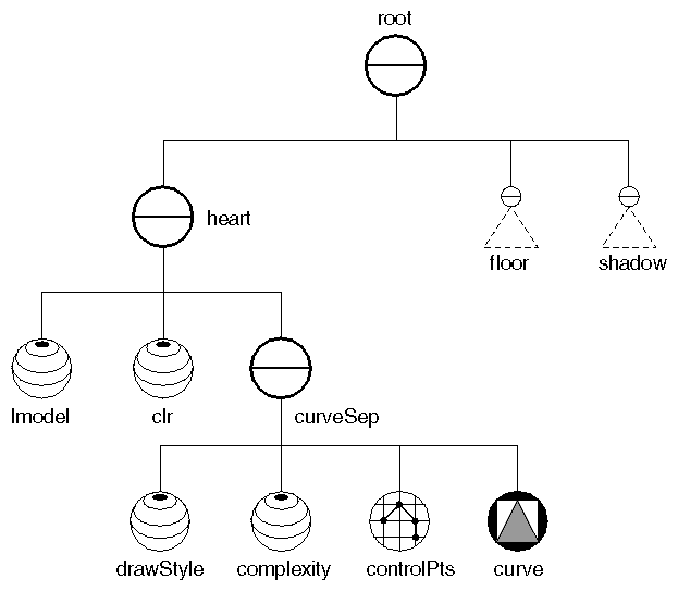
Figure 8-11 shows the scene graph for the nodes in this example. Figure 8-12 shows the resulting curve.
// The control points for this curve
float pts[7][3] = {
   { 4.0, -6.0,  6.0},
   {-4.0,  1.0,  0.0},
   {-1.5,  5.0, -6.0},
   { 0.0,  2.0, -2.0},
   { 1.5,  5.0, -6.0},
   { 4.0,  1.0,  0.0},
   {-4.0, -6.0,  6.0}};

// The knot vector
float knots[10] = {1, 2, 3, 4, 5, 5, 6, 7, 8, 9};

// Create the nodes needed for the B-Spline curve.
SoSeparator *
makeCurve()
{
   SoSeparator *curveSep = new SoSeparator();
   curveSep->ref();
|
// Set the draw style of the curve. SoDrawStyle *drawStyle = new SoDrawStyle; drawStyle->lineWidth = 4; curveSep->addChild(drawStyle); // Define the NURBS curve including the control points // and a complexity. SoComplexity *complexity = new SoComplexity; SoCoordinate3 *controlPts = new SoCoordinate3; SoNurbsCurve *curve = new SoNurbsCurve; complexity->value = 0.8; controlPts->point.setValues(0, 7, pts); curve->numControlPoints = 7; curve->knotVector.setValues(0, 10, knots); curveSep->addChild(complexity); curveSep->addChild(controlPts); curveSep->addChild(curve); curveSep->unrefNoDelete(); return curveSep; } |
Example 8-2 creates a uniform B-spline curve that passes through the end control points. The knot sequence has a multiplicity of 4 at the beginning and end, which causes the curve to pass through the first and last control points. In between, the curve is uniform.
The scene graph for the nodes in this example has the same structure as the scene graph shown in Figure 8-11. “A Uniform B-Spline Curve that Passes through the Endpoints” shows the resulting curve.
// The control points for this curve
float pts[13][3] = {
   { 6.0,  0.0,  6.0},
   {-5.5,  0.5,  5.5},
   {-5.0,  1.0, -5.0},
   { 4.5,  1.5, -4.5},
   { 4.0,  2.0,  4.0},
   {-3.5,  2.5,  3.5},
   {-3.0,  3.0, -3.0},
   { 2.5,  3.5, -2.5},
   { 2.0,  4.0,  2.0},
   {-1.5,  4.5,  1.5},
   {-1.0,  5.0, -1.0},
|
   { 0.5,  5.5, -0.5},
   { 0.0,  6.0,  0.0}};

// The knot vector
float knots[17] = {
   0, 0, 0, 0, 1, 2, 3, 4, 5, 6, 7, 8, 9, 10, 10, 10, 10};

// Create the nodes needed for the B-Spline curve.
SoSeparator *
makeCurve()
{
   SoSeparator *curveSep = new SoSeparator();
   curveSep->ref();

   // Set the draw style of the curve.
   SoDrawStyle *drawStyle  = new SoDrawStyle;
   drawStyle->lineWidth = 4;
   curveSep->addChild(drawStyle);

   // Define the NURBS curve including the control points
   // and a complexity.
   SoComplexity  *complexity = new SoComplexity;
   SoCoordinate3 *controlPts = new SoCoordinate3;
   SoNurbsCurve  *curve      = new SoNurbsCurve;
   complexity->value = 0.8;
   controlPts->point.setValues(0, 13, pts);
   curve->numControlPoints = 13;
   curve->knotVector.setValues(0, 17, knots);
   curveSep->addChild(complexity);
   curveSep->addChild(controlPts);
   curveSep->addChild(curve);

   curveSep->unrefNoDelete();
   return curveSep;
}
|
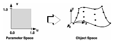
A surface differs from a curve only in that it has two parametric directions (u and v) instead of one (Figure 8-14), and that the order and knot vector must be specified for both parameters.
The two parametric dimensions, u and v, are mapped to 3D object space. As with curves, control points are specified in object space. The u and v parameters can have a different order, and a different knot sequence, although they are often the same. The order for each dimension is specified as
order = number_of_knots - number_of_control_points
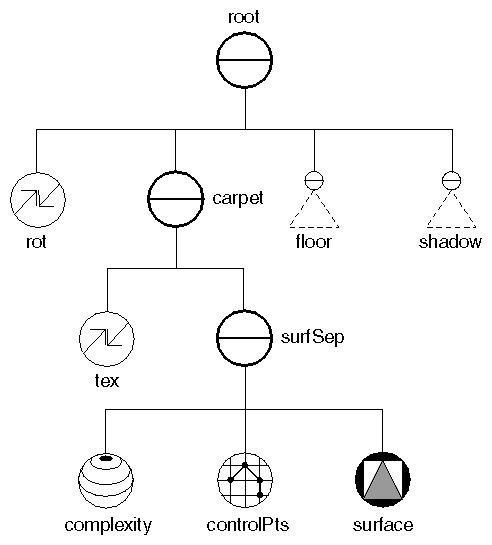
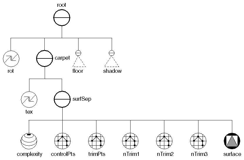
Example 8-3 creates a plain Bezier surface. The knot vectors define a cubic Bezier surface (multiplicity 4 at beginning and end). The surface is order 4 with 16 control points arranged in a four-by-four grid. The u and v knot vectors each have a length of 8. Figure 8-15 shows the scene graph for the nodes in this example. Notice that the points used as control points (controlPts) must precede the NURBS node (surface) in the scene graph. “Bezier Surface” shows the rendered image.
// The control points for this surface
float pts[16][3] = {
   {-4.5, -2.0,  8.0},
   {-2.0,  1.0,  8.0},
   { 2.0, -3.0,  6.0},
   { 5.0, -1.0,  8.0},
   {-3.0,  3.0,  4.0},
   { 0.0, -1.0,  4.0},
   { 1.0, -1.0,  4.0},
   { 3.0,  2.0,  4.0},
   {-5.0, -2.0, -2.0},
   {-2.0, -4.0, -2.0},
   { 2.0, -1.0, -2.0},
   { 5.0,  0.0, -2.0},
   {-4.5,  2.0, -6.0},
   {-2.0, -4.0, -5.0},
   { 2.0,  3.0, -5.0},
   { 4.5, -2.0, -6.0}};

// The knot vector
float knots[8] = {
   0, 0, 0, 0, 1, 1, 1, 1};
|
// Create the nodes needed for the Bezier surface.
SoSeparator *
makeSurface()
{
   SoSeparator *surfSep = new SoSeparator();
   surfSep->ref();

   // Define the Bezier surface including the control
   // points and a complexity.
   SoComplexity  *complexity = new SoComplexity;
   SoCoordinate3 *controlPts = new SoCoordinate3;
   SoNurbsSurface  *surface  = new SoNurbsSurface;
   complexity->value = 0.7;
   controlPts->point.setValues(0, 16, pts);
   surface->numUControlPoints = 4;
   surface->numVControlPoints = 4;
   surface->uKnotVector.setValues(0, 8, knots);
   surface->vKnotVector.setValues(0, 8, knots);
   surfSep->addChild(complexity);
   surfSep->addChild(controlPts);
   surfSep->addChild(surface);

   surfSep->unrefNoDelete();
   return surfSep;
}
|
 | Tip: If a NURBS surface is changing, inserting an SoComplexity node with SCREEN_SPACE specified as the type may improve performance, especially if the NURBS surfaces are far away. |
Profile curves are used to trim (cut areas away from) a NURBS surface. Profile curves themselves are not rendered; they are simply used to trim any subsequent NURBS surfaces in the scene graph. Like transformations, profile curves are pushed and popped by separator groups, yet they accumulate with each other.
Profile curves are often used to perform a stencil operation, such as cutting a shape out of a cloth surface with a pair of scissors. They are also used to remove sharp corners from a NURBS surface. See also Example 6-3, which uses a profile curve with 3D text.
Trimming NURBS surfaces is considered an advanced topic. If this is your first exposure to a NURBS, experiment first with curves and surfaces, then move on to trimmed surfaces.
A profile curve can consist of a linear profile curve (SoLinearProfile), a NURBS curve (SoNurbsProfileCurve), or a combination of the two. For coordinates, it uses either SoProfileCoordinate2 (for nonrational profile curves) or SoProfileCoordinate3 (for rational profile curves). The main requirement is that the composite profile curve make a complete loop, with its first point repeated as its last point. In addition, it cannot be self-intersecting.
 | Tip: If you want your profile curve to be straight but follow the surface, use an SoNurbsProfileCurve with an order 2 curve. (See Example 8-4.) Linear profiles create straight trim edges in object space that do not follow the surface. You will seldom use an SoLinearProfile to trim a NURBS surface. |
The direction in which the points of a profile curve are defined is significant. If the profile curve is defined in a clockwise direction, the area inside the curve is discarded and the area outside the curve is retained. If the profile curve is defined in a counterclockwise direction, the area inside is retained and the area outside is discarded. Profile curves can be nested inside each other but cannot intersect each other. The outermost profile curve must be defined in a counterclockwise direction (see Example 8-4).
Profile curves are defined in parameter space, which is mapped to
object space.
Example 8-4 adds profile curves to the surface created in Example 8-3. Figure 8-17 shows the scene graph for the nodes in this example. Notice that the points used as control points (controlPts) must precede the NURBS node (surface) in the scene graph. Similarly, the points that define the profile curve (trimPts) must precede the profile-curve nodes (nTrim1, nTrim2, and nTrim3). And, naturally, the profile-curve nodes must precede the NURBS surface to be trimmed.
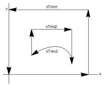
Figure 8-18 shows the trim curves used in Example 8-4, mapped in parameter (u/v) space. This example uses three NURBS profile curves. Each curve has its own knot vector. The first curve, nTrim1, has four segments and five control points (it starts and ends at the same point). It is an order 2 curve that passes through the endpoints. The second profile curve, nTrim2, is also linear. It passes through the endpoints and has three segments. The third profile curve, nTrim3, is a cubic curve (order = 4). It has a multiplicity 4 at beginning and end (which makes it a Bezier curve that passes through the endpoints).
Notice that these trim curves are nested inside each other and that the outermost curve is counterclockwise. They do not intersect each other. “A Trimmed Bezier Surface” shows the trimmed Bezier surface produced by Example 8-4.
// The array of trim coordinates
float tpts[12][2] = {
   {0.0, 0.0},
   {1.0, 0.0},
   {1.0, 1.0},
   {0.0, 1.0},
   {0.2, 0.2},
   {0.2, 0.7},
   {0.9, 0.7},
   {0.9, 0.2},
   {0.7, 0.0},
   {0.4, 0.8}};

// The 16 coordinates defining the Bezier surface.
float pts[16][3] = {
   {-4.5, -2.0,  8.0},
   {-2.0,  1.0,  8.0},
   { 2.0, -3.0,  6.0},
|
   { 5.0, -1.0,  8.0},
   {-3.0,  3.0,  4.0},
   { 0.0, -1.0,  4.0},
   { 1.0, -1.0,  4.0},
   { 3.0,  2.0,  4.0},
   {-5.0, -2.0, -2.0},
   {-2.0, -4.0, -2.0},
   { 2.0, -1.0, -2.0},
   { 5.0,  0.0, -2.0},
   {-4.5,  2.0, -6.0},
   {-2.0, -4.0, -5.0},
   { 2.0,  3.0, -5.0},
   { 4.5, -2.0, -6.0}};

// The 3 knot vectors for the 3 trim curves.
float tknots1[7] = {0, 0, 1, 2, 3, 4, 4};
float tknots2[6] = {0, 0, 1, 2, 3, 3};
float tknots3[8] = {0, 0, 0, 0, 1, 1, 1, 1};

// The Bezier knot vector for the surface.
// This knot vector is used in both the U and
// V directions.
float knots[8] = {0, 0, 0, 0, 1, 1, 1, 1};

// Create the nodes needed for the Bezier patch
// and its trim curves.
SoSeparator *
makeSurface()
{
   SoSeparator *surfSep = new SoSeparator();
   surfSep->ref();

   // Define the Bezier surface including the control
   // points, trim curve, and a complexity.
   SoComplexity  *complexity     = new SoComplexity;
   SoCoordinate3 *controlPts     = new SoCoordinate3;
   SoNurbsSurface *surface       = new SoNurbsSurface;
   complexity->value = 0.7;
   controlPts->point.setValues(0, 16, pts);
   surface->numUControlPoints.setValue(4);
   surface->numVControlPoints.setValue(4);
   surface->uKnotVector.setValues(0, 8, knots);
   surface->vKnotVector.setValues(0, 8, knots);
   surfSep->addChild(complexity);
   surfSep->addChild(controlPts);

   SoProfileCoordinate2 *trimPts = new SoProfileCoordinate2;
   SoNurbsProfile *nTrim1        = new SoNurbsProfile;
   SoNurbsProfile *nTrim2        = new SoNurbsProfile;
   SoNurbsProfile *nTrim3        = new SoNurbsProfile;
   long trimInds[5];

   trimPts->point.setValues(0, 12, tpts);
   trimInds[0] = 0;
   trimInds[1] = 1;
   trimInds[2] = 2;
   trimInds[3] = 3;
   trimInds[4] = 0;
   nTrim1->index.setValues(0, 5, trimInds);
   nTrim1->knotVector.setValues(0, 7, tknots1);
   trimInds[0] = 4;
   trimInds[1] = 5;
   trimInds[2] = 6;
   trimInds[3] = 7;
   nTrim2->linkage.setValue(SoProfile::START_NEW);
   nTrim2->index.setValues(0, 4, trimInds);
   nTrim2->knotVector.setValues(0, 6, tknots2);
   trimInds[0] = 7;
   trimInds[1] = 8;
   trimInds[2] = 9;
   trimInds[3] = 4;
   nTrim3->linkage.setValue(SoProfile::ADD_TO_CURRENT);
   nTrim3->index.setValues(0, 4, trimInds);
   nTrim3->knotVector.setValues(0, 8, tknots3);

   surfSep->addChild(trimPts);
   surfSep->addChild(nTrim1);
   surfSep->addChild(nTrim2);
   surfSep->addChild(nTrim3);
   surfSep->addChild(surface);

   surfSep->unrefNoDelete();
   return surfSep;
}
|
The following texts provide more detailed information on NURBS curves and surfaces:
Bartels, R., J. Beatty, and B. Barsky, An Introduction to Splines for Use in Computer Graphics and Geometric Modeling. Los Altos, Ca.: Morgan Kaufmann, 1987.
Farin, G., Curves and Surfaces for Computer Aided Geometric Design, 2e. San Diego, Ca.: Academic Press, Inc., 1990.
